Blog

I've published a new video about how I've made my procedural mountain forest bigger, better and faster over the past two years:

Links to things mentioned in the video

My previous video about my procedural mountain forest.

My LayerProcGen framework and my talk about it at Everything Procedural Conference 2024.

My free game The Cluster (full trailer), which my LayerProcGen framework was originally developed for.

My blog post about the procedural creatures I alluded to.

The GPU Instancer Pro (Asset Store) third party tool I use for GPU instancing with frustum and occlusion culling.

The Grasslands - Stylized Nature (Asset Store) model pack I use for my new trees.

My blog post about my Point Cloud Sound technique.

My blog post about the game progression dependency graphs I alluded to.

My erosion filter video and blog post. The links section at the end of the blog post has links to implementations by others in various engines, tools, and games.

A GitHub Gist demonstrating shared C# and shader code.

My blog post about atmospheric perspective and distant mountains.

Frequently asked questions

The trees are popping. Could you fade them in instead?
Not very easily. The trees already use dither-based fading between the tree LOD levels. When you see trees pop into existance, it's because a terrain chunk is replaced with terrain chunks of a more detailed LOD level that has denser tree coverage. Fading the new trees in when this happens would require having an additional fading feature on top of the one used for tree LOD levels. Not only would it make the tree shaders more complex, it would also be a lot of work to route the required data into all the tree instances. It would require changes to GPU Instancer Pro third party tool I'm using, or else I'd have to use it in a significantly more low-level way. Either way, it's frankly beyond my skill level, as I'm not nearly as proficient with shader "data plumbing" as I am with shader math.

This blog post and the companion video both explain an erosion technique I’ve worked on over the past eight months. The video has lots of elaborate animated visuals, and is more focused on my process of discovering, refining, and evolving the technique, while this post has a bit more implementation details on the final iteration. I suggest watching the video first, but it’s not required. You can also skip right to the links at the end.

In the real world, rainfall on mountains tends to converge into water streams and rivers, which carve gullies in the mountain sides. These gullies may form branching patterns, as smaller water streams merge into larger ones. And the gullies often butt up against each other, leaving sharp ridges dividing them.

But when generating virtual landscapes, the simulation of countless water drops is slow. It’s not very suitable for generation in chunks either, which means it’s not practical to use when generating landscapes that are too large to generate all at once.

This means techniques are sought after, which can produce the appearance of erosion without having to deal with simulating the process of it. This post is about such a technique.

It’s essentially a special kind of noise which produces gorgeous branching gullies and ridges, while still allowing every point to be evaluated in isolation, which means it’s fast, GPU-friendly, and trivial to generate in chunks.

Furthermore, rather than defining the landscape entirely, it can be applied on top of any height function, essentially applying erosion on top as a filter.

Background

There’s a website called Shadertoy where people create and share standalone shaders. A shader is a program that runs on the GPU, which can be used to determine what a virtual surface should look like, or for various other effects, or even entire scenes.

In 2018 a user called Clay John (Bluesky) posted a Shadertoy called Eroded Terrain Noise. He wrote:

This shader is the result of a long time dreaming of a noise function that looked like eroded terrain, complete with branching structure, that could be run in a single pass pixel shader. I wanted to avoid anything simulated because then you cannot easily make infinite terrains.

That dream sounds familiar, but Clay John actually made it work. His Shadertoy is the original version of this technique. Hats off to him.

Later, in 2023, a user called Fewes, aka Felix Westin (website), posted a Shadertoy which built on top of the one by Clay John. Fewes’ version slightly tweaked how the erosion effect worked, and presented it in a vastly more polished way.

In 2025 to 2026 I’ve implemented my own versions of the technique. First I made a version that addresses a few shortcomings of the original technique, and has more intuitive parameters. Eventually I developed a version that works in a completely different way, which produces crisper gullies and ridges and has more expressive parameters. But before going over the differences, let’s start with the basics of the original technique.

The basic idea

We start with a height function where we know not just the height at each point, but also the gradient, meaning the direction and steepness of the steepest ascent. Water flows in the opposite direction, so you can think of the negative gradient at each point as an arrow showing the direction that water would flow down the slope.

Let’s start simple, with a slanted surface, where the gradient is the same everywhere.

We use the gradient to add stripes that run along this direction. The stripes produce alternating gullies and ridges, that could plausibly have been created by water eroding the terrain.

The sides of these gullies and ridges come with their own gradients, which are added to the original to produce new combined gradients.

We can then repeat the whole thing again at a smaller scale: Add smaller stripes which run along the new slopes. These form new gullies and ridges which naturally branch out at an angle from the first ones.

By convention, each repetition is called an octave. Add a few more octaves, and we should be done, right?

Except – it’s not quite as simple as I just made it sound.

If we apply the erosion to our original height function, where the gradient is not the same everywhere, we get a chaotic mess. Even if we show it with just a single octave, it’s still full of chaotic gullies that are often not aligned with the slopes at all. What’s going on?

Generating stripes

To rotate the stripe pattern, we have to choose some pivot point to rotate it around.

The problem is the rotation around this pivot point will create increasingly large distortions in the output the further away from the pivot point we are. This is because changes in the rotation angle not only changes the direction of the stripes at a given point, but also shifts which stripe is under that point.

The approach used in the erosion implementation is to divide the pattern into cells that each have their own pivot point for the stripes. If you imagine a square grid, there’s one cell per grid square, with its pivot placed randomly inside the square, similar to simple Worley noise.

We still get a bit of distortion, but it’s not too bad, since the pivot point is never too far away. At least as long as the gradient of the height function doesn’t change too drastically within a single cell.

To ensure smooth results without discontinuities, we blend the stripes of neighboring cells. The stripes are essentially extruded sine waves, specifically a cosine wave for the height offset and a sine wave for the derivative (slope).

The reason the stripes blend so nicely together even when not aligned, is that if you blend two unaligned sine waves, you just get a new sine wave with a smaller amplitude.

The cell size has a big effect. If we choose a cell size that’s large compared to the stripe width, we get significant distortion issues, just like when we used a single pivot point. If we choose a small cell size, there’s barely room for any stripes, and we get a kind of grainy noise instead.

If we make the cell size even smaller relative to the stripe thickness, the pattern begins to be all white. Or in terms of ridges and gullies, it’s all ridge and no gully. This is because each cell uses a stripe pattern with a white stripe in the center.

Preserving peaks

When I talk about peaks and valleys, I’m referring to the local maxima and minima of the original height function, whereas when I talk about ridges and gullies, I’m referring to the local maxima and minima of the gully stripes applied in each octave of the erosion filter.

Now that we can generate stripes aligned with any gradient, we can apply our erosion effect to the height function without getting chaotic distortions.

However, although we’ve now got nice gullies on the mountain sides, the mountain peaks look wrong. They barely look like peaks at all.

That’s because the peaks may be located anywhere in our stripe pattern, and they get arbitrarily lifted or lowered based on that. Furthermore, there’s an issue whenever the surface steepness approaches zero, which happens at peaks and valleys. When the slope is zero, the gradient has no defined direction, so the direction of the gradient changes abruptly around those spots, which creates chaotic stripe patterns in the surrounding area.

There are two ways we can address this, and both are based on the steepness of the slopes. There’s the original approach used by Clay John and Fewes, which I call the frequency approach, and there’s an alternative approach I came up with, which I call the fade approach.

The frequency approach

The original approach used by Clay John and Fewes is to make the stripe frequency proportional to the slope, so the stripes are thicker, the flatter the terrain is.

At peaks and valleys, where the steepness is zero, the stripes become infinitely thick. And because each cell has a white stripe in the center, this means mountain peaks and valleys, where the slope is zero, always land on the part of the stripe pattern that corresponds to a ridge, and never a gully.

This works great for mountain peaks, but I discovered that it unfortunately causes valleys to have bulges at the bottom, since they land on "ridges" in the stripe pattern too. This is not visible in their Shadertoys, because they have faded out the erosion at lower altitudes. And this workaround is great if you want smooth valleys.

However, if you apply the erosion at equal strength everywhere, the bulges at valleys appear, and it means you can’t get crisp, V-shaped valleys.

You can find my Shadertoy here based on the frequency approach. It’s similar to the one by Fewes, but is refactored to have more intuitive parameters.

The fade approach

I came up with a different approach, which is to keep the stripe widths consistent and instead fade out the stripes where the steepness approaches zero. If we fade towards "white" – the maximum value of the gully octave – we get a similar effect as with the frequency approach, that the shape of peaks is preserved, but there are bulges at the bottom of valleys.

Now, if we fade towards "black" instead – the minimum value of the gully octave – we don’t get any bulge at the valleys, but instead we get a crease at the peaks. But if we fade towards a value that goes from black at mountain valleys to white at mountain peaks, we can get nice crisp peaks and valleys at the same time.

In my implementations, I let it be up to the user to supply this fade target value as an input parameter to the erosion function, for example based on altitude.

For a height value h at the current point, it could look like this, if the expected height range goes from valleyAlt to peakAlt:

float inverse_lerp(float a, float b, float v) {
    return (v - a) / (b - a);
}

// Convert the altitude to a value between -1 and 1.
float fadeTarget =
    inverse_lerp(valleyAlt, peakAlt, h) * 2.0 - 1.0;

The fade approach has a different issue that needs to be carefully handled. It initially seemed to create visible folds – also called discontinuities – caused by abrupt changes in the gradient directions around the peaks and valleys. But I later found out that this can be addressed by using an appropriate shaping function on the slope.

From early on, I had been raising the steepness of the slope to a power of 0.5, which is equivalent to taking the square root of the slope. This applies erosion more evenly than if we used the slope directly. Unfortunately it produces sharp discontinuities at peaks and valleys. This is because the square root curve starts off vertically, so as the slope increases from zero to even the tiniest slant, the erosion immediately increases drastically.

But there are many other functions we can use to shape the erosion. The one I ended up using is to flip the curve vertically by subtracting it from one, then raising it to a power of two, and then flipping the result back.

float ease_out(float t) {
    // Flip by subtracting from one.
    // The saturate function clamps between 0 and 1.
    float v = 1.0 - saturate(t);
    // Raise to a power of two and flip back.
    return 1.0 - v * v;
}

This has a somewhat similar shape as the square root – in fact it’s mirrored around the diagonal – but the curve starts off much more moderately. This mostly removes the appearance of discontinuities, especially when we layer multiple octaves of gullies.

With this tweak, the fade approach works just as well as the frequency approach. And unlike the frequency approach, it works well when applying the erosion at full strength everywhere, which can be used to create sharp V-shaped valleys, if desired.

The quest for crisp, branching gullies

The erosion we’ve got so far looks nice, but the larger gullies and ridges get a little bit lost in the smaller ones. I’d prefer if the gullies at all scales could have crisper ridges and creases, and more clearly show a branching pattern.

To address this, I did a lot of experimentation, and developed three techniques that go hand in hand. I call them stacked fading, normalized gullies, and straight gullies, and I’ll go over each of them in the next sections.

Stacked fading

We already fixed a problem with crispness earlier. The mountain peaks and valleys didn’t look crisp until we began fading towards black or white for the valleys and peaks respectively. And it turns out we can do something similar for the gullies and ridges.

Let’s establish a few terms first.

I’m calling the value we fade towards the fade target and it’s generally expressed in a variable that goes from -1 at valleys to 1 at peaks.

Then there’s the amount we’re fading towards the fade target. We’re doing a weighted average (also known as a lerp or a mix) of the gullies and the fade target, which can be 100% gullies at steep slopes, 100% fade target at flat terrain, or some mix of the two, depending on the slope. We can think of this as a mask applied to the fade target, before we layer it on top of the gullies.

When we’ve been talking about the fade approach, the fade target and mask have been based on the original height function and its slopes. But just like we don’t want gullies right on top of the mountain peaks or valleys, we also don’t want smaller gullies right on top of the ridges or creases of larger gullies. We can achieve this if we conclude each octave by updating the mask and fade target to also be black and white at that octave’s creases and ridges.

The diagram above may seem daunting, but here’s the gist of it:

• The octave 1 raw gullies are faded towards the input fade target based on the input mask to produce the octave 1 faded gullies. You can think of it as the masked fade target being "overlaid" on top of the octave 1 raw gullies. Nothing new so far.
• The octave 1 faded gullies are then used as the new fade target for the next octave. The mask is also updated: From the octave 1 raw gullies, a mask contribution is created which is opaque at the creases and ridges, where the slope is zero. The existing mask is layered on top of the new mask contribution to produce the new combi-mask after octave 1.
• The same steps are repeated for each new octave. The octave 2 raw gullies are faded towards the new fade target based on the new combi-mask to produce the octave 2 faded gullies. These are used as the new fade target, and the mask is updated with a new contribution based on the octave 2 raw gullies. And so on.

In broad terms, each new octave adds more ridges and creases to the terrain surface, which increasingly restricts the surface area where subsequent gullies can have any influence on the surface.

How are new mask contributions combined with the existing combi-mask? Let me start by saying that it was easiest in the diagram above to conceptualize the mask as being applied to the fade target, but in the code it’s actually a mask applied to the gullies, so 0 means all fade target and 1 means all gully. In this form, the new mask contribution can simply be multiplied onto the combi-mask to produce the new combi-mask.

We can furthermore implement a useful control here. By raising the inverse of the combi-mask (meaning its complement) to some power before multiplying it with the new contribution, we can control how detailed the erosion looks. Lower values restrict the effect of higher frequency gullies to steeper slopes.

float pow_inv(float t, float power) {
    // Flip, raise to the power, and flip back.
    // The saturate function clamps between 0 and 1.
    return 1.0 - pow(1.0 - saturate(t), power);
}

combiMask = pow_inv(combiMask, detail) * newMask;

Normalized gullies

One thing that’s holding back crisper ridges and creases is the inconsistent magnitude of the gullies, caused by the interpolation of stripes that may or may not be well aligned.

At one point I realized that since we interpolate both cosine and sine waves in parallel, we can think of each cosine/sine pair as a point on a unit circle, and the interpolated value as a point on a circle too. The interpolated circle point may have shrunk to a radius smaller than one, but it’s trivial to normalize it back to one. And this in turn means that both the interpolated cosine and sine waves have a consistent magnitude of one.

Now, in the actual interpolated stripe function we’ve used up until this point, the sines are multiplied with a vector orthogonal to the terrain gradient in order to calculate the gradient of the slope. But since this vector is the same for all contributing samples, the multiplication can be postponed and applied to the interpolated result rather than to each contributing sample, leaving us free to perform the normalization first.

When straightforward normalization is applied, some curious artifacts appear where ridges and creases join up and form loops. Supposedly, this happens at points where the interpolated waves cancel out completely; something that seems to unavoidably happen with some regularity. On the terrain, this manifests as spiky protrusions (and holes).

However, the loopy artifacts can be avoided if we only normalize lengths above a certain threshold. To avoid discontinuities between normalized and non-normalized gullies, we can use the following approach:

• Scale lengths by a factor k that’s larger than one.
• Clamp resulting lengths to one.

I’ve used a factor k of 2, such that lengths greater than 0.5 become normalized. This produces a good tradeoff with lots of gullies of consistent magnitude and without loopy artifacts.

The style of partial normalization I’ve chosen produces second order discontinuities (abrupt changes in slope) in some places, but as it’s not noticeable once multiple octaves are used, I haven’t bothered with a more sophisticated approach.

I figured that the ability to produce directional noise is useful for many other purposes than erosion, so I’ve released the noise function as Phacelle Noise, which I’ve written about here.

Straight gullies

Once the ridges and creases got more crisp, another issue became apparent. Smaller ridges and creases would often run along larger ones for a little distance before branching out.

It’s here that the limitations of modeling gullies as extruded sine waves becomes apparent. See, on the side of gullies, the terrain slope is strongly affected by it, pointing sideways away from the ridges. But at the bottom and top of gullies, they have virtually no effect on the terrain slope. So at those points, smaller gullies will simply run parallel to the larger ones.

Since the effect is gradual, smaller gullies tend to curl at the ends, rather than branching off cleanly from the larger gullies. A visualization of the ridges and creases with just two octaves of gullies shows the difference clearly.

The effect of non-straight gullies is more subtle on the actual terrain surface. But when carefully comparing the images below, you may find that the first one, which does not have straight gullies, has more instances of ridges with small grooves on top, less instances of gullies branching out at clean angles rather than curving, and an overall texture which feels a bit more stringy and smushy.

I fixed the issue of non-straight gullies by essentially faking consistent slopes when calculating the slopes used for the gully stripe pattern directions.

We can pretend that the slope of a gully is constant from top to bottom, as if the gullies were extruded triangle waves instead of sine waves. The faked slope is implemented by using the sign of the sine wave that controls the gully slope, rather than using its value directly. That is, if the sine is negative, we use a value of -1, and otherwise a value of 1.

I also tried making the gullies actually be extruded triangle waves, but due to complex interactions in how the different octaves combine, that just ended up looking worse.

One aspect of the overall erosion technique I haven’t explicitly covered yet is that it outputs not only the heights of the eroded terrain, but also the analytical derivatives. However, those derivatives were never very accurate, whether in Clay John and Fewes’ implementations or my own. They are used internally to calculate the gully directions, but the output derivatives were never actually used for anything.

But even if not accurate, they can still come in handy, so I don’t want to remove support for them. (I actually did begin using them to calculate tree coverage.)

With the fade approach, the mask is also used on the derivatives of each octave. They are faded towards a slope of zero rather than the fade target value, which is only relevant for heights. But fading the derivatives towards zero at ridges and creases undermines the straight gullies technique.

So I began calculating derivatives in two different ways in parallel. The output derivatives are stored as part of a heightAndSlope variable whereas the internal version is stored in a gullySlope variable. And while the former is faded towards zero according to the mask, the latter is not.

The faked gully slope does mean that the new straight gullies created based on it have discontinuities at the creases and ridges of the faked slopes, as stripes going in different directions butt right up against each other. This can be seen in the octave 2 raw gullies part of the diagram from earlier.

But these discontinuities are fully faded away in the faded gullies used for the output height offset (and output derivatives), so they’re not a problem.

One issue with the slopes remains. For the gullies, we could pretend they’re triangle waves, and calculate the slope of those pretend-triangle-waves according to the frequency and magnitude, but not so with the slopes of the input heights, of which we can assume very little.

If we use the input slope unchanged, the initial gully octave will have a disproportionally large effect near the peaks and valleys, where the input heights are typically rounded and thus have little to no slope contribution. But in the eroded output terrain, the peaks and valleys are typically pointy, with just as steep slopes as elsewhere.

I’ve experimented with a variety of solutions to this, but in the end what produced the best results was to just pretend that the input heights have a specific slope everywhere. This pretend slope can be tweaked to somewhat match the typical slope the eroded terrain ends up having.

It’s a bit ironic that my early work on the erosion technique was focused on making the analytical derivatives more accurate, only to end up giving up on that entirely. But that’s just how a labyrinthine process of discovery sometimes goes.

New coat of paint

The technique has now changed sufficiently that some tweaking of the parameters is in order, to make the most of the new functionality. While at it, I also found a new spot in the heightmap to focus on. Below is the reference terrain I’ll use going forward, which also includes features covered in the remainder of this article.

While not part of the erosion technique itself, it’s also fun to dress up the terrain with nice materials. I’ve been tweaking the logic inherited from the Shadertoy by Fewes, and added bumpy parts to it that evokes trees too. Furthermore, I managed to add little streaks that evoke water drainage using a technique I’ll discuss further down.

Pointy peaks

It turns out that normalizing the gullies make the mountains less pointy, keeping more of the rounded shape of the input height function.

At first, I tried to compensate by applying a special function to the input height that made peaks more pointy, prior to passing them to the erosion function. But I later found that there is a simpler solution that can be trivially implemented in the erosion function itself: Simply scale down the gullies part of the faded gullies by some gully weight factor (such as 0.5) and compensate by scaling up the erosion strength by the inverse factor (like 2.0).

Pointy peaks are still dependent on the fade target having a value close to 1.0, so in all the example images, the peaks at lower altitudes are less pronounced.

We can look at what happens when the gully weight is reduced to zero. This preserves the overall shape of the eroded mountains, including crisp peaks and valleys, but without all the gullies.

There is a subtle kind of ghosting effect of the gullies present, where ridges and creases alike are turned into all ridges where the original fade target is positive, and all creases where it’s negative. This unhelpfully counteracts half of the intended creases and ridges if very low gully weight values are used, but at larger values there are no noticeable issues.

There are undoubtedly other ways to go around this, but the approach here is simple and works well enough.

Rounding of ridges and creases

The implemented technique can produce very sharp ridges and creases, but something not quite as sharp is often desired. For example:

• Real mountain peaks and ridges tend to not be razor sharp if you zoom in sufficiently.
• Valleys and the bottom of gullies can get a rounded shape if sediment builds up in them.

For this reason I implemented "edge rounding" with separate control for creases and ridges. As I’ve previously touched upon, the mask is based on the slope passed through a shaping function. By chaining a variable-size ease-in function onto this shaping function, rounding of the ridges and creases can be achieved. And by mixing two different rounding values – one for ridges and another for creases – based on the fade target, the amount of rounding can be controlled separately for those.

I wanted the rounding to have the same size for gullies of all octaves, so the rounding values are counter-adjusted in accordance with the erosion lacunarity value, which controls how much smaller the gullies are in each octave (typically half the size).

The rounding also affects peaks and valleys stemming from the original height function (and its slopes), but the erosion function doesn’t know about the sizes of the terrain features coming from those, so an input value is provided for tweaking the rounding of those.

Water drainage

While getting the erosion increasingly crisp, the idea of a holy grail occurred to me: Could the technique model the branching gullies so crisply that it could render little branching river networks? It turns out: Kind of, with some caveats.

Side note: I later learned that the branching streaks on mountain sides I had in mind constitute dendritic drainage, which, apart from rivers and creeks, also include channels of snow, sediment, and debris-flow. The colored streaks are often not the water itself, but the leftover rocks and sediment which is colored differently from the surrounding soil or vegetation. Either way, it tends to look like bright lines.

If we ignore the recently discussed gully weights and ridge and crease rounding, then the fade target is practically already a map of the ridges and creases in the eroded terrain, once the technique has gone through all the gully octaves. Only, the last octave appears with much thicker lines than the rest, since it hasn’t been filtered through the mask. This can be resolved by fading it towards a neutral value of zero / gray based on the mask, resulting in what I call a ridge map.

Now, those recently discussed features do undermine the ridge map, so in order to avoid having to choose between one and the other, we can keep track of two copies of the fade target and mask in parallel, and process the ones for the ridge map without those features.

Here’s a visualization of the ridge map on the terrain:

With the ridge map, it’s easy to draw little lines at the bottom of all the gullies that resemble dendritic drainage. Here’s the image of the textured terrain again:

It’s not a perfect solution, since the interpolated stripes we use for the gullies cannot consistently produce unbroken lines. So sometimes a gully, and the drawn water drainage at its bottom, just stops halfway down a mountainside rather than following through all the way down to the lowest reachable point. Nevertheless, it looks nice and can be sufficient for use cases that don’t require accuracy in this regard.

Future work

You can see my final iteration of the technique in my Shadertoys Advanced Terrain Erosion Filter and Mouse-Paint Eroded Mountains.

As has hopefully been clear, the erosion technique I’ve described in this post is highly malleable. Compared to the original version by Clay John and Fewes, I’ve modified it to a point where its internal workings, capabilities, and characteristics are entirely different.

While I don’t have plans to further work on this technique myself, I find it likely that others will, given how open-ended the nature of the technique is, and how ripe it is with potential.

In my work with the technique, I’ve simply aimed to make the eroded terrain look good to my eyes, loosely using a bunch of reference images for inspiration.

An interesting jumping off point for future work could be to try to use the technique to emulate a variety of specific eroded terrain types, each based on different references. The input parameters should allow for a wide variety of looks on their own, especially when considering most of them can be varied based on other variables. If the technique then falls short of being able to emulate certain terrain characteristics, that could point the way towards potential future improvements.

I’ve released my code under the Mozilla Public License v2 in order to encourage further sharing of improvements. I’m looking forward to seeing how the technique evolves in the future!

Based on feedback after publication I've added some additional notes after the links section.

Links

YouTube videos

Some things are easier to explain in motion.

• My video Fast & Gorgeous Erosion Filter Explained has more elaborate visualizations than this blog post, and more details on the initial process I went through.
• Better Mountain Generators That Aren’t Perlin Noise or Erosion on Josh’s Channel is a highly polished and well explained video on two other non-simulated erosion techniques. I reference this video in my own video.

Shadertoys

You can run and see these visuals directly in your browser, and easily see and modify the source shader code too.

• Eroded Terrain Noise by Clay John (Bluesky). The original version of the technique.
• Terrain Erosion Noise by Felix Westin (Fewes) (website). Slightly tweaked erosion effect, and presented in a vastly more polished way.
• Clean Terrain Erosion Filter by me. My earlier rewrite of Clay John and Fewes’ technique (based on the frequency approach), with more intuitive parameters.
• Advanced Terrain Erosion Filter by me. My final iteration of the technique, with animated parameters.
• Mouse-Paint Eroded Mountains by me. My final iteration of the technique, with interactive mouse painting of the terrain.
• Phacelle Noise Animation by me. A demonstration of the Phacelle Noise I extracted into a self-contained function (blog post here).

Erosion filters in the wild

Let me know if you use the erosion filter technique in your project and have public images or videos to show for it!

I'm very happy so many people have found the technique useful enough to make their own implementations in a variety of shapes and forms. Some of the ones below are faithful implementations, while others are partial, derived, or based on an earlier version of the technique.

Implementations in tools, engines, and online

• Highly customizable online demo of the erosion filter and terrain (faithful to my Shadertoy) by optozorax
• Implementation in Unity Burst posted on Reddit and released on Github by Luke Mitchell.
• Implementation in Unity Shadergraph posted on Bluesky and released on Github by Jens Maier.
• Implementation in Unreal's landmass plugin posted on Twitter by Michael Kinsey.
• Implementation in Godot posted (with source) on Godot forum by Henry.
• Implementation in Blender geometry nodes Quick Erosion Filter free Gumroad download by Jérémy Derlande (Kollapse3D).
• Implementation in Houdini blog post with source files by eetu.
• Implementation in Leveller heightmap modeler tool included in version 4.4 (with source) by Ray Gardener.
• Online standalone web widget to apply the erosion filter to a PNG by Robert Winslow

Implementations in games and private experiments

• Implementation in Hytale's Worldgen v2 posted on Bluesky and released on Github by Verday.
• Minecraft published mod and source on GitHub by oovaa8.
• Erosion on a sphere posted on Mastodon by metarapi.
• Terraform Blending Test YouTube video by HerrLynnsTube.
• |peak| implementation in Desmos graphing calculator graph by lemon (and a simpler version here).

Shadertoy video exporters

This is not entirely related to erosion techniques, but here are the tools I used to render high quality Shadertoys footage for the video. Okay, I may also be using the links section here to tell a side story about my video production woes.

• Shadertoy Exporter (original) by Jonathan Giroux (Koltes). This tool worked great, until it broke when the Shadertoy website introduced Cloudflare human verification in early October 2025.
• Shadertoy Exporter (forked) by Lara Davidova (larathedev). This fork was made to work with the Cloudflare human verification, and was briefly functional, until the Shadertoy website entirely disallowed being displayed in an iframe later in October 2025.
• Shadertoy Exporter (Godot version) by krazyjakee (NodotProject). This rewrite based on Godot is partially functional at the time of writing. It’s Windows-only, and (for me) has the following bugs: Does not convert the rendered frames into videos, has to be restarted after each render, and frequently does not register text input until the window focus is switched away and back. I begrudgingly used this for later footage in the video, manually running ffmpeg on the frames.
• I’m aware there are also frame exporter browser plugins for Firefox and for Chrome, but these have even worse usability for me. I have my browser set to display a save dialog when downloading a file, so when I try to render a Shadertoy for 200 frames, it opens 200 save dialogs.

Additional notes

On using the second derivatives (curvature) for the fade target

Several people have suggested using the second derivatives (curvature) instead of the altitude for the fade target.

Using altitude is indeed not robust in the general case, since e.g. some valley could be higher up than some mountain peak. I'm not sure there's a perfect solution, and I kind of let it be up to the user to decide what to base the input fade target parameter on. I just base it on altitude in all my demonstrations.

I did think about using the second derivatives (curvature), but then every function involved in producing the input heights has to calculate and return those second order derivatives, or alternatively it has to be done numerically which is either slow (via multi-sampling) or rather inaccurate (via shader derivatives).

On top of that, curvature does not produce a value that's between -1 and 1 as the fade target needs, so you'd have to combine it with other things (like the first derivatives) to wrangle it into a useful range. That's absolutely possible, but hand-tweaking the particulars may still be needed.

So while it's something I considered, I don't really have a good solution. I'm curious if others will find a better way to handle this.

For my game The Big Forest I want to have creatures that are both procedurally generated and animated, which, as expected, is quite a research challenge.

As mentioned in my 2024 retrospective, I spent the last six months of 2024 working on this – three months on procedural model generation and three months on procedural animation. My work on the creatures actually started earlier though. According to my commit history, I started in 2021 after shipping Eye of the Temple for PCVR, though my work on it prior to 2024 was sporadic.

Though the creatures are still very far from where they need to be, I'll write a bit here about my progress so far.

The goal

I need lots of forest creatures for the gameplay of The Big Forest, some of which will revolve around identifying specific creatures to use for various unique purposes. I prototyped the gameplay using simple sprites for creatures, but the final game requires creatures that are fully 3D and fit well within the game's forest terrain.

Another year went by as an indie game developer and what do I have to show for it?

In last year's retrospective I wrote that apart from working on my game The Big Forest in general, I had four concrete goals for 2024:

• Present my Fractal Dithering technique
• Release my Layer-Based ProcGen for Infinite Worlds framework as open source
• Wrap up and release The Cluster as a free experimental game
• Make better use of my YouTube channel

I ended up doing only two of those, but it was the two most important ones to me, so I'm feeling all right with that.

Release of LayerProcGen as open source

I released my LayerProcGen framework as open source in May 2024. LayerProcGen is a framework that can be used to implement layer-based procedural generation that's infinite, deterministic and contextual.

I wrote extensive documentation describing not only the specifics of how to use it, but also the overarching ideas and principles it's based on. I also did a talk at Everything Procedural Conference about it, which was well received.

In 2022 I came up with some new ideas for what kind of game The Big Forest (working title) could be. During the year, I developed a way to procedurally create dependency graphs and also procedurally create fully playable game levels based on the graphs.

The Cluster is finally released and available for free on Itch. It's a 2.5D exploration platformer set in an open world that's carefully procedurally planned and generated, and does a few interesting things I haven't yet seen in other games (check out the links for more info).

Here's a trailer:

My last blog post about The Cluster was in 2016 and titled "Development of The Cluster put on hold", and by that I meant put on hold indefinitely.

2023 was a pretty good year for me!

I'll touch here briefly on my personal life, then go on to talk about the Quest 2 release and sales of Eye of the Temple, and finally talk about my new game project and goals for 2024.

Personal life

It's the first year since the pandemic that didn't feel affected by it. I moved from Denmark to Finland in 2020, just as the pandemic began, so on the social side it was some slow years initially.

Things picked up in 2022, but especially in 2023 we had lots of family and friends from Denmark visit us here and have a great time, and we also made more strides on the local social network front.

Particularly memorable was a wonderful weekend celebrating the 40th birthdays of me and a friend, with some of my closest family and friends from Denmark and Finland at a site called Herrankukkaro in the beautiful Finnish archipelago.

Eye of the Temple released on Quest and turned a profit

In April 2023, a year and a half after the original PC release on Steam, my VR game Eye of the Temple was finally released for Quest 2, with the help of Salmi Games. While it was super tough getting there, in the end we managed to ship the game at a level of quality I'm very proud of. Others agreed; it got a great critical reception, as well as a high user rating of 4.7 out of 5 stars.

It's super gratifying regularly seeing new reviews of the game from people who say it's the best VR experience they've had. Oh, and recently, UploadVR ranked it the 5th best game for Quest 3 and Screen Rant ranked it the 6th best game for Quest 2. Wow, what an achievement for my little game! (But remember, critical acclaim does not equal sales…)

I’m no longer working on the game at this point. After being occupied with it over a span of seven years, I really want to move on, and I'm also done with VR in general for now. But the sales of the game are still developing, so let's talk a bit about that.

My thinking about the game’s sales performance has changed a lot over time. I didn't pay myself a regular salary during the game’s three years of full time work. But when evaluating the game financially, I use the old salary from my previous job as reference, and calculate whether my time investment at that salary (I’ll refer to it as just “my investment”) would be covered retroactively by the game’s revenue. Of course, I also keep in mind that the covered percentage would be higher if I based it on a more moderate salary.

I was initially slightly disappointed in the Steam sales. As I wrote about back in November 2021, the projected year one sales would only cover 25% of my investment. Back then I expected the Steam year one revenue to make up the majority of the game's lifetime revenue. One year later, the sales had outperformed that projection, and my investment was actually covered 40%.

A lot has happened since then, in particular due to the Quest launch.

Comments from many VR developers in 2021 and 2022 had indicated that Quest sales could commonly be 5x-10x as large as Steam VR sales. For Eye of the Temple, the Quest week one revenue was merely twice of what the Steam week one revenue had been, so it was not quite as high as Salmi Games and I had hoped for. Speaking with other VR developers in 2023, it seems that the time when Eye of the Temple launched on Quest was generally a bad period for Quest game sales.

Still, Quest is easily the most important VR platform, and later the sales picked up significantly, with the recent Black Friday and Xmas sales combined having as big an impact on revenue as the launch sales. Already, 70% of total revenue has come from Quest and 30% from Steam, with the Quest version having been out for a shorter time.

My investment is now covered 140%. In other words, even based on a proper salary for myself that's fitting for my experience, Eye of the Temple has recently flipped well into profitability. That still doesn't make it a runaway hit, but it's really nice to know that it's a success not only creatively and as a passion project, but also in terms of financial sustainability. Back in 2020 when I was still developing the game, I had not expected that at all for my first commercial title.

Today is the one year anniversary of the release of my VR adventure Eye of the Temple on Steam! It's currently 40% off to celebrate.

I thought I'd take a moment to talk about what I've been up to since the release, both related to Eye of the Temple and other projects.

The Cluster is an exploration platformer game I've been developing in my spare time for some time. You can see all posts about it here.

As of the time being, I've put development of The Cluster on hold indefinitely.

Burdens

After having worked on the game for more than ten years (!) I finally came to the conclusion that the overall design and constraints in the game is making it very hard for me to finish it, while also holding me back from trying out a lot of otherwise interesting ideas.

• The game is procedural and the same every time you play, which makes it super important to guarantee you can't get stuck.
• There is gravity and no ability to fly, which means you will get stuck unless the algorithms are carefully designed to make it impossible. It has to be more or less mathematically provable.
• The AI enemies can follow you practically everywhere, which means every obstacle needs to be coded to also be usable by AI.
• The world is constructed from a rather large-scale grid which makes things like large ramps and hills impossible (just a bit boring).
• The third-person perspective require art and animation resources for avatar and enemies.
• The side-scrolling format makes it hard to wordlessly attract the player to interesting things in the far distance, because only the immediate environment can be seen. This creates more of a reliance on maps and narratives to explain the reasoning for seeking out those far away things, and that plays against the procedural nature of the game.

Now, none of those things are impossible to overcome, and I did have a playable demo at the end of 2015 that worked under all of those constraints. But the game is not yet nearly varied enough, and every new feature is very tough to pull off under the burden of all those constraints.

Focusing on my strengths

I've switched focus to working on projects that I hope both play more to my strengths, and should be possible to pull off in a shorter time frame.

• First-person perspective without jumping, so no fiddly physics.
• No humanoid characters, which decreases the demands for art, animation and "behaviors".
• No ambition of a story (some of my favorite games don't have one anyway).

This frees me up to focus more exclusively on making interesting environments, which is what I'm most passionate about.

The good news is that the time has not been entirely wasted. For one, I've learned a LOT. And for another I've developed several pieces of substantive tech that are fully reusable in my future projects.

Speaking of future projects, I'm working on a few already.

One is The Big Forest, though I'm not actively working on it right now. The focus here is to create nice, interesting and varied environments with very simple gameplay on top. I want it to me my own favorite walking simulator. In its current early stage it's already one of the best virtual forest experiences I've had.

The project I'm actively working on is a VR game for Vive that I've tweeted a little bit about and will soon announce properly here on the blog.

Stay tuned!

I've been continuing my work on the procedural terrain project I wrote about here. I added grass, trees and footstep sounds (crucial!) and it's beginning to really come together as a nice forest to spend some time in.

I made a video of it here. Enjoy!

If you want to learn more about it, have a look at this thread on the procedural generation subreddit.

In the beginning of 2014 I was interested in procedurally generating computer games puzzles with typical elements like toggles, gates that can be triggered to open, boxes or boulders that can be moved onto pressure plates, etc. Many games contain elements like these and I took inspiration in particular from the game Lara Croft and the Guardian of Light.

To better understand these puzzles, and understand what makes a puzzle interesting or boring, I started creating a tool for analyzing and visualizing the state space of the puzzle. In the Procedural Content Generation mailing list I discussed the approach here.I've worked on it on and off since, and while I still don't have an algorithm for procedurally generating the puzzles, the tool itself is interesting in its own right. It's called PuzzleGraph and I've just released it for free.

Get PuzzleGraph at itch.io

You can setup and connect puzzle elements like gates, toggles, pressure plates and boulders, and see the state space of the puzzle visualized, including solution paths, dead ends and fail states.

If you make some puzzles with PuzzleGraph, I'd love to see them!

The best demonstration is this video I made. If you already saw the video, skip down a bit for some new info and announcements.

Pathfinding is not just for finding paths for AI agents/NPCs and similar. It’s also for procedurally creating paths.

While working on path creation for a procedural terrain, I had the problem that the generated paths would keep having too steep sections, like this:

It was too steep and also didn’t look natural at all. I kept increasing the cost multiplier for slopes, but it didn’t help.

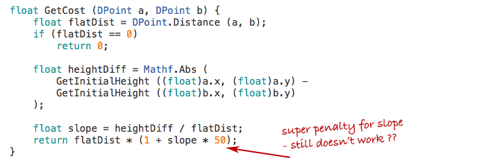
Then it hit me: My function just penalized the vertical distance, but it didn’t make any difference if this vertical distance came gradually or all at once.

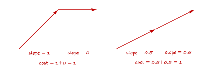
So in fact, my cost function wasn’t trying to avoid steepness - rather it was trying to make a path where the altitude changes monotonically. It would do everything it could to avoid the path first going up and then down again.

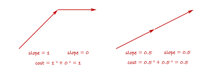
But I didn’t care if the path went a little up and down, as long as it wasn’t too steep at any point. To achieve this behavior, I needed to penalize steep slopes more than linearly, for example by squaring it.

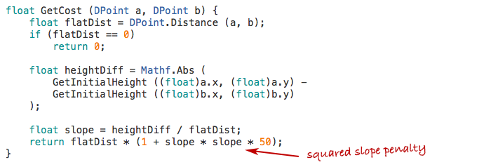
This has the effect of penalizing abrupt changes in altitude and reward gradual changes.

And sure enough, after the change the generated paths avoided steepness and looked much more like what humans would create.

Tweaking pathfinding cost functions is one of those odd little things that I really enjoy. Seeing a little change in a formula imbue a generated creation with what could be mistaken for human design is really fascinating and fun!

Further notes

The observation-turned-blog-post in its original form ended there, but I've compiled some further notes for those who want to dig into the details.

Pathfinding method

Let me tell about the method I use for the pathfinding, since I was asked about this. I won't do an introduction to pathfinding in general here but assume understanding of the principles of performing pathfinding using an algorithm like A* or similar on a graph of nodes connected by edges.

Such a graph can be represented in many ways. Sometimes it's a data structure with explicit data representing all the nodes and edges and how they're connected. Other times it can just be a grid (like a 2D array) and each cell is implicitly connected to the neighboring cells - maybe the 4 or 8 neighbors, depending on whether diagonal connections are used.

It doesn't really matter, and a pathfinding algorithm can typically easily be modified to work with one or the other. Apart from giving it a start node and goal node, the important part is that you can tell the algorithm:

• Which other nodes are a node connected to?
• What is the real or estimated cost of getting from one node to another?

You might have data for this stored in advance or you might calculate the answers on the fly when asked.

For the terrain pathfinding I do the latter. In fact, there is neither an explicit graph, nor any 2D array. There is no data structure at all for the pathfinding to happen inside. Instead, it's all implicit, based solely on coordinates. I tell the pathfinder what the start and end coordinates are, and there's a function for getting "neighbor coordinates" to a given coordinate. There's also a function for getting the cost of getting from one coordinate to another, as you saw earlier.

This may sound completely free-form and magical at first, but there still is a structure that must be adhered to. You must imagine a grid structure and ensure the coordinates always fall within this grid. In my case it's a plain quadratic cell grid where each cell has a size of 5. So the start coordinate, goal coordinate, and every provided neighbor coordinate must always have x and y values that are multiples of 5. You also shouldn't use floating-point numbers for this, since they can produce floating point precision errors, and even the slightest imprecision can cause the pathfinding to completely fail.

I wanted my paths to be able to have a natural, non-jagged look, so I wanted edges to come in 16 directions instead of the basic 8. The 8 additional directions are achieved by going two cells out and one to the side. This provided me with an interesting choice of whether the 8 other directions should also go two cells out, or just one.

In theory the second option can be weird, since if you need to move just one cell the path have to first side-step by two cells. But in practice both seems to work fine. The first images in this post were made with the first option but I later decided to use the second to avoid the path having very small-scale zig-zags.

Effects of different parameter values

I got asked on the proceduralgeneration sub-reddit:

How rapidly does the path change as you increase the power from 1.0 to 2.0? What happens if you go past 2.0? Does the path eventually have to spiral around the mountain or something?

I had actually been content just using the values I had found which seemed to work well enough, but now that I'd been asked, of course I wanted to find the answers too! I tried doing the pathfinding with the power values 1.5, 2.0 and 3.0 and with the multiplier values 1, 2, 3, 4, 5, 6, 7, 10, 15, 20, and 25. I had moved the multiplier inside the power function since the original version of the code, so those multipliers are multiplied onto the steepness before the resulting value is raised to the given power. Here's a table of the results.

Some notes on the result.

Overall the common theme is that the results range from straight and boring to wildly tortuous. At the extreme end, the path begins to create loops - something that should be impossible with path-finding. However, the edges I use in the path-finding can cross each other. This means that they can appear to loop even though they never pass through the same points from the perspective of the path-finding. They only begin to do this once the path-finding is so extremely sensitive to tiny changes in altitude that the small difference in altitude between one of two crossing edges is enough for it to exploit it to loop around. I should say that I only sample the altitude at the end-points of each edge, which appears to be fully sufficient except in the extreme cases like this.

Note that there are very similar occurrences across the different power values. For example, multiplier 10 at power 1.5 looks just like multiplier 6 at power 3.0, and multiplier 7 at power 2.0 looks just like multiplier 5 at power 3.0. Does this mean that any result you can get with one power value, you can also get with another? That there exists a transformation that means they're mathematically equivalent? No, I don't believe so. It feels like there's subtle differences. For example, the progression of paths with power value 3 begins to do loops before it begins to take a major detour, while for power value 2, the loops only start happening after it has begun doing a large detour. The differences are very subtle though and hard to put the finger on exactly.

One thing that's tempting to look for is qualitative differences, such as some paths doing many small zig-zags and others doing larger swoops. However, I think that's a red herring. The algorithms doesn't measure sharpness of turns or frequency of turns in any way and shouldn't be able to tell one from the other. I think that the seeming qualitative differences are thus up to unpredictable aspects of how the path-finding interacts with the terrain height function that sometimes just happen to produce one result or the other. To answer it in terms of the original question: If the terrain was perfectly conical, a path from the base to the top might equally well form a spiral, a zig-zag pattern, or any other combination of left-winding and right-winding sections.

My own pragmatic takeaway from this is that sticking with just a power value of 2 seems fine and I'd then use multiplier values between 3 and 15 depending on how straight or tortuous I want the path to be.

Perspectives

These generated paths were a proof-of-concept for a new project I'm working on and I'm sure I'll learn more as I go along. For example, already I'm learning some things about approaches for flattening the terrain around the paths which I may share at a later point when I'm a bit more sure of my findings. For now, I hope you found this useful!

2024 update: Code available

I've now released a framework called LayerProcGen as open source, and one of the sample scenes generates natural paths using the technique described in this article. So a fully functional implementation is now available for study and use.